
Model Details
As an avid hiker, undercast conditions (where the clouds are below you) are quite a treat. They’re also often unexpected. While the surprise can be fun, hiking in a white-out isn't as fun when you could have gone tree skiing instead. As such, and in an attempt to avoid doing actual work, I set out to predict undercast conditions in New Hampshire’s White Mountains.
I began this project assuming I could grab cloud base height information from existing weather reports (such as Windy), and use that to forecast undercast conditions. 10's of research papers, 1000's of lines of code, and more dead ends and stupid mistakes than I'd care to admit, here we are.
I quickly discovered that undercast conditions are far more complex than a simple temperature inversion. In the section below, I use data from six weather models (HRRR, RAP, NAM, GFS, ECMWF, and NBM), training three different machine learning models (Random Forest, Gradient Boosting, and XGBoost), after a simpler physics-based approach failed.
About Undercasts
While academic literature about undercast skies is sparse (it’s almost like climate scientists have something more important to study), there is a general consensus on what conditions are needed to produce undercast skies.
First and foremost, a temperature inversion is required, where temperature increases with height (rather than decreasing), trapping a cold layer of air at lower temperatures.
The following are good references on undercast conditions:
- ScienceDirect: Atmospheric study (S016980951930941X)
- Boundary-layer meteorology article (Springer)
- What is a cloud inversion? — EatSleepWild
- Mount Washington Observatory — Undercast
- Green Mountain Club — Temperature inversion & undercast
Determining if it’s undercast
To validate any model (ML or otherwise), we need to know if it was actually undercast. While I would prefer to just hike up Mt. Washington every day and collect data myself; I also would like to finish my PhD at some point, so we need a different solution.
Step 1 — Determine undercast conditions from the webcam
The Mt. Washington Observatory has multiple live summit webcams. They publicly archive ~2 years of footage, containing a daily image taken at noon. I analyzed every single image by hand, assigning it a label as undercast or not. Fun fact: manually categorizing 1000 images (2 years x 2 webcams) by hand was not fun.
That gives 589 labeled days spanning 25 May 2024 to 3 January 2026, of which 22 are undercast.
22 positive examples are nowhere near enough. Certainly not to train a classifier, and even difficult for a physics-based approach (eg. looking at local forecasts for conditions that drive undercasts).
Step 2 — Determine undercast conditions from the METAR report
Mount Washington is one of the few remaining staffed weather stations in the country. Every hour, a human, or cat, on the summit augments the station’s METAR report. These additional, man-made comments often contain information about cloud conditions. A key remark that appears in many undercast reports is TPS LWR — “tops lower” — which gives the coverage and the top height of any cloud deck sitting below the 6,288 ft summit.
An example report might read:
This observation viewer shows 42 of these reports next to the webcam frames taken at the same time. The sample is not random, but instead has similar number of undercast (and non-undercast) days.
Thus, we want to determine which of the METAR remarks best correspond to undercast conditions, and will use the ~600 webcam-labeled dates to do so. That search produced five cuts/conditions:
| Condition | Why |
|---|---|
TPS LWR coverage is broken or overcast | At least 5/8 of the sky below the summit is cloud covered. "Scattered" cloud conditions didn't contain enough clouds to be considered undercast. |
| visibility > 40 SM | If visibility is too poor, then the summit is likely at least partially in the clouds. |
| no ceiling overhead, or one at or above 5,000 ft | A low lid overhead makes it more of a sandwich, than a true undercast. Is this "sandwich" is small enough, two layers blend together. |
| deck top at least 500 ft below the summit | If the clouds are too close to the summit, it no longer looks like an undercast, and you're mostly in the clouds. |
| lowest layer of any coverage overhead at or above 1,000 ft | The ceiling test only looks at broken and overcast layers, so it'll pass a report carrying FEW002 — cloud touching the summit. Even a few clouds directly at summit elevation can obscure a view. |
What each cut does (individually)
These cuts were not the first thing I tried, nor were they generated randomly. The impacts of each cut are shown below.
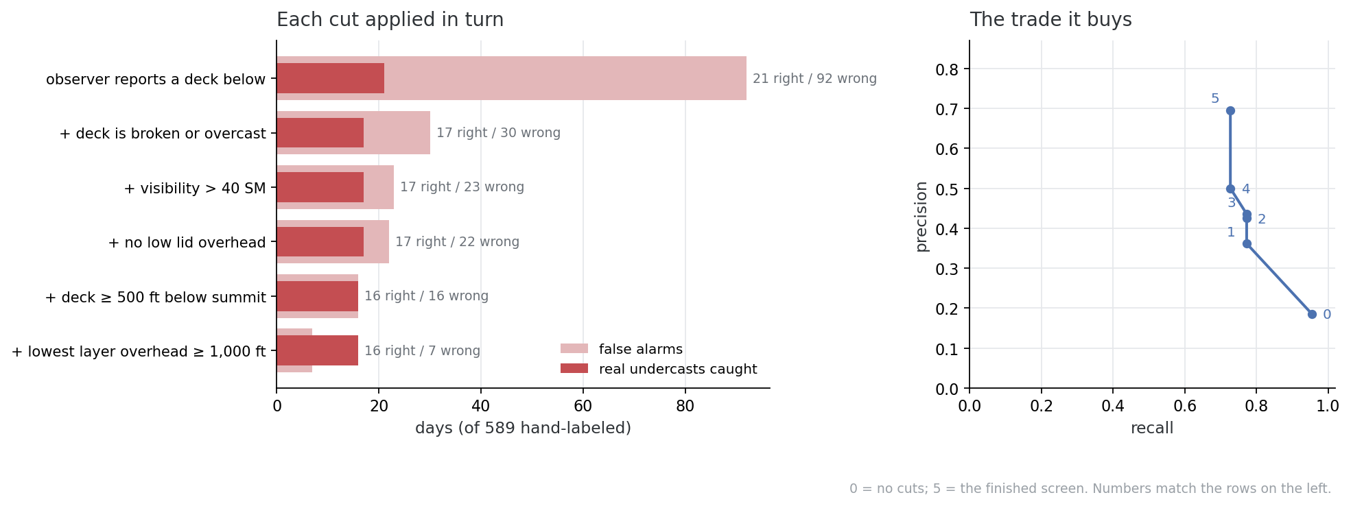
Starting from “the observer mentioned a deck below the summit” and adding one condition at a time. Almost all of the recall is present at the start; the job of the cuts is to strip out false alarms without taking real days with them.
The impact of each cut individually (not after other are applied), is shown below.
| Drop this one cut… | Extra false alarms | Extra real days caught | Precision | Verdict |
|---|---|---|---|---|
| broken or overcast coverage | +25 | +4 | 0.38 | Does the heavy lifting, but it is the one real trade — it costs four genuine undercast days. |
| lowest layer overhead ≥ 1,000 ft | +9 | 0 | 0.50 | The best cut in the set. Removes nine false alarms and does not cost a single real day. |
| deck ≥ 500 ft below summit | +3 | 0 | 0.62 | Modest but free. |
| visibility > 40 SM | +1 | 0 | 0.67 | Nearly redundant here — the other cuts have already removed almost everything it would catch. |
| no low lid overhead | +1 | 0 | 0.67 | Earns almost nothing on this sample. It stays because the sandwich case it guards against is real and these are only 22 days. |
Scored against the full 589 hand-labeled days, the finished cuts have a precision of 0.70 and recall of 0.73. That is, when it says undercast it’s right about 70% of the time, and it catches about 73% of the real undercasts.
Those are numbers are determined by webcam interpretations, so it is worth looking at the actual webcam images. This gallery shows every labeled day that reported a deck below the summit, grouped by what the cuts did with it — what passes, what each cut throws out, and which of the discarded days were real undercasts after all.
Step 3 — Run the cuts over 29 years
We now have an adequate way of determining if it was undercast from METAR remarks. It's not great, but good enough, given we started with 22 undercast examples. Applying the undercast cuts to the 253,317 hourly observations from 1997 through 2026, 6,852 pass as undercast. That's over 300 times more than from manually labeling webcam images.
One caveat: the undercast rate is not constant over time (click to expand)
The fraction of METAR observations passing the cuts climbs over time. While it's possible that this is a rare positive consequence of anthropogenic climate change, it's probably just reporting bias. When we look at the rate of reports mentioning clouds decks TPS LWR, we see that the rate of reporting also increased. The data is noisy, given the low statistics, but the increase in undercast observations appears to be consistent with an increase in cloud deck reporting.
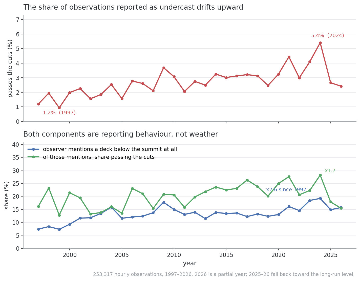
We have to be careful here, especially when training ML models. Without correction, a model would learn that recent years have more undercasts. The fix is in how the comparison cases are chosen — every undercast observation is matched against non-undercast observations drawn from the same year, same month, and same hour of day, so the calendar and the clock carry no signal and the weather parameters have to do the work.
Our final training set
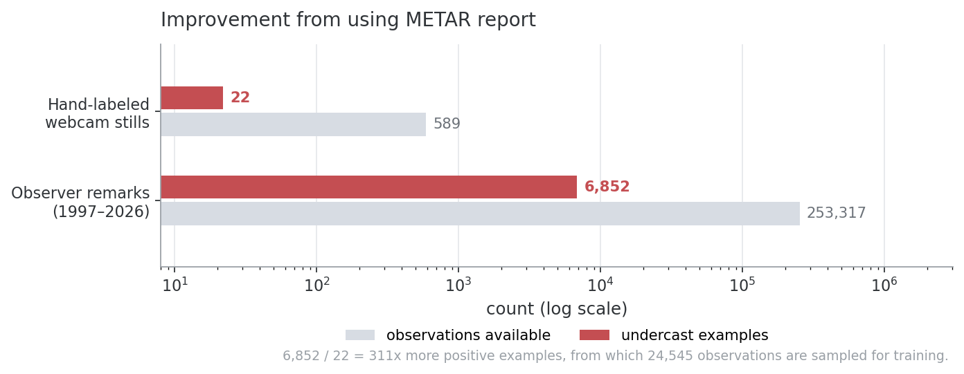
Hand-labeling almost two years of webcam frames produced 589 days carrying 22 undercast examples. By contrast, using METAR observation remarks increased the record to 253,317 hourly observations carrying 6,852 — over 300× more positive examples, and enough that a classifier can see more than a handful of cases.
First Attempt: Simple Physics-based cuts
Scientific consensus is that undercast conditions are caused by temperature inversions. Initially, I figured it would be easy to query a couple of NOAA weather models, look for when temperature inversions were predicted, and voila, I have an undercast predictor. No fancy techniques required.
Turns out, predicting localized weather patterns is hard; especially in the mountains; especially on the most prominent peak for almost 1,000 miles; and especially on a mountain renowned for its harsh and unpredictable weather.
Based on my understanding of uncercast conditions, I came up with a couple conditions that I hoped would correlate strongly with undercasat conditions.
| Rule | In words |
|---|---|
| A inversion | Temperature at 850 mb warmer than at 925 mb. That layer sits just below the summit, so a positive difference is a capping inversion exactly where an undercast’s lid should be. |
| B summit above the deck | The model reports no cloud ceiling, or one above 1,917 m — i.e. the summit isn't in a cloud. |
| C = A and B | An inversion, with the summit out of it. |
| D = C and sees far | Plus modelled surface visibility above a threshold — if you can't see very far, you're in a cloud. |
How they do
Scored on the base-rate holdout (a full unsampled year). In the sample, undercast occurs ~3% of the time:
| Source | Best rule | Precision | Recall | False alarms |
|---|---|---|---|---|
| Random sampling | Fire at random, as often as HRRR’s rule D does | 0.03 | 0.21 | 1,751 |
| HRRR | D | 0.09 | 0.60 | 1,651 |
| NAM | D | 0.07 | 0.53 | 1,879 |
| RAP | D | 0.07 | 0.48 | 1,743 |
| GFS | C | 0.07 | 0.44 | 1,604 |
| ECMWF | A (no ceiling field published) | 0.06 | 0.68 | 1,975 |
While the physics-based approach works (it's about 3x better than random guessing), it's still not particularly useful. 3 times a small number is still a small number. Before abandoning this approach, we can investigate why it fails.
Two cuts that I expected to work, but didn't (click to expand)
“Requiring a cloud top below the summit.”. Rows where HRRR puts the cloud top below 1,917 m have a 9.2% undercast rate against a 16.8% base rate in that sample, while rows where HRRR reports no cloud at all run at 21.5%. This is backwards! Low-lying clouds in the HRRR forecast result in fewer undercasts!
I assume that this is due to HRRR's 3km resolution. Variables like temperature and wind may be easier to model than cloud formation in narrow valleys.
“A high percentage of Low cloud cover.” Adding a low-cloud-fraction term makes every combination worse — F1 on the training split drops from 0.41 to 0.09. I assume this is also driver by the resolution.
Both failures likely have a similar cause. The pressure-level temperatures are trustworthy here because a pressure surface is not as sensitive to the terrain; anything keyed to height above the model’s ground requires high granularity spacial resolution, which none of these models have (everything is on order of multiple km).
It becomes clear why these cuts fail when you look at the underlying distrubutions, separated by METAR-labeled undercast vs. non-undercast. These plots show the inversion strength, ceiling, visibility and boundary-layer depth for undercast hours against everything else, and lets you step through individual days model by model.
There are some clear patterns here (most notably the inversion plot); however the distributions overlap enough that no simple threshold can easily separate them.
So, you have some high-dimensional data with non-trivial correlations between parameters; let's throw some ML at it and see what sticks!
Developing the ML Model
Thanks to the METAR text, we now have a labeled dataset for training our machine learning model. Now we have to select parameters and a model.
Input parameters
(click to expand)
Weather models such as HRRR, RAP, NAM, GFS, ECMWF, and NBM contain hundreds of parameters. Not all of these are relevant to undercast predictions. The following are used (each is pulled from every model that provides it). They were selected based on what a dumb physicist thought seemed relevant. Many are strongly correlated with one another. Parameter importance is shown later for different models.
| Key | Description |
|---|---|
| cloud_top | Cloud top height (AGL). The altitude of the highest extent of a cloud layer, useful for identifying deep convection or storm tops. |
| boundary_layer_cloud_layer | Boundary layer cloud cover (%). Total cloud fraction within the planetary boundary layer, the lowest ~1–2 km of the atmosphere. |
| low_cloud_layer_percent | Low cloud cover (%). Fractional cloud coverage below ~2 km (~6,500 ft), typically stratus or stratocumulus. |
| middle_cloud_layer_percent | Mid-level cloud cover (%). Fractional cloud coverage between ~2–6 km (~6,500–20,000 ft), typically altocumulus or altostratus. |
| high_cloud_layer_percent | High cloud cover (%). Fractional cloud coverage above ~6 km (~20,000 ft), typically cirrus or cirrostratus. |
| cloud_ceiling_m | Cloud ceiling height (meters AGL). The height of the lowest broken or overcast cloud layer, critical for aviation and visibility assessment. |
| cloud_base_m | Cloud base height (meters AGL). The altitude of the bottom of the lowest cloud layer, closely related to the Lifted Condensation Level (LCL). |
| cloud_top_pres | Cloud top pressure (Pa). The atmospheric pressure at the top of the cloud layer — lower pressure = higher altitude cloud tops. |
| cloud_base_pres | Cloud base pressure (Pa). The atmospheric pressure at the base of the cloud layer, an alternative vertical coordinate to height. |
| cloud_top_hgt | Cloud top geopotential height (meters). Similar to cloud_top but expressed as geopotential height rather than AGL, more consistent across terrain. |
| wind_10m_day_max | Daily maximum 10m wind speed (m/s). The peak wind speed at 10 meters above ground over the forecast day, useful for fire weather and wind advisories. |
| tmp_500mb | Temperature at 500 mb (~5,500 m). Mid-troposphere temperature, used to assess atmospheric instability and identify cold upper-level troughs. |
| tmp_700mb | Temperature at 700 mb (~3,000 m). Lower-mid troposphere temperature, important for identifying warm/cold advection and orographic effects. |
| tmp_850mb | Temperature at 850 mb (~1,500 m). Low-level temperature commonly used as a proxy for surface airmass character and snow level estimation. |
| tmp_925mb | Temperature at 925 mb (~750 m). Near-surface temperature just above the boundary layer, useful for detecting inversions and cold air damming. |
| tmp_1000mb | Temperature at 1000 mb (~100 m). Near sea-level temperature, representing conditions very close to the surface in low-elevation areas. |
| tmp_2m | 2-meter air temperature (°C). Standard screen-level temperature used in most surface weather forecasts and human comfort assessments. |
| rh_2m | 2-meter relative humidity (%). Moisture content of the air at screen level, directly relevant to fire weather, fog formation, and human comfort. |
| hpbl_surface | Planetary boundary layer height (meters). The depth of the turbulent mixing layer above the surface — higher in the afternoon, lower at night and during inversions. |
| hgt_0C_iso | Height of the 0°C isotherm (meters). The freezing level altitude, critical for determining rain/snow transitions and icing conditions. |
| vis_surface | Surface visibility (meters). Forecast horizontal visibility at the surface, reduced by fog, precipitation, smoke, or dust. |
| prate_surface | Instantaneous precipitation rate (kg/m²/s). The rate of precipitation at a given forecast hour, useful for identifying intensity of ongoing precip. |
| apcp_surface | Accumulated total precipitation (kg/m²). Cumulative precipitation over the forecast period, equivalent to mm of liquid-equivalent rainfall. |
The forecast models
(click to expand)
Undercast is predicted for six independent weather models. Each one gets its own dedicated ensemble, and a seventh combined model draws on the parameters of all six at once.
| Model | What it is | Scale / resolution | Cloud fields |
|---|---|---|---|
| HRRR | High-Resolution Rapid Refresh | 3 km · CONUS · short-range | Yes |
| RAP | Rapid Refresh (HRRR's parent model) | 13 km · regional | Yes |
| NAM | North American Mesoscale | 12 km · regional | Yes |
| GFS | Global Forecast System | ~0.25° · global medium-range | Yes |
| ECMWF | Integrated Forecasting System (open data) | ~0.25° · global | Dynamics / thermodynamics only |
| NBM | National Blend of Models (statistical blend) | CONUS blend | Yes — incl. probabilistic ceiling & visibility |
| Combined | Every model's parameters together | — | — |
Model selection & training
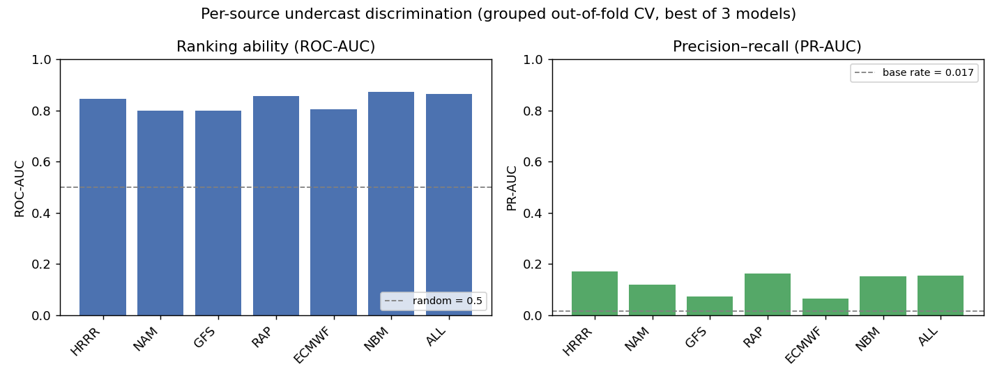
Three (XGBoost, Random Forest and Gradient Boosting) algorithms are trained independently for each of the seven weather model combinations above. You're only as good as your training data, and given the uncertainty in the undercast labeling technique, I'd have a hard time justifying any algorithms fancier than these vanilla-ML ones. Undercast conditions are rare (~3%), so the classes are heavily imbalanced. Rather than synthesizing samples, each one handles that with class weights (Random Forest’s balanced class weights, XGBoost’s scale_pos_weight, balanced sample weights for Gradient Boosting).
ML for idiots — what those three algorithms actually do (click to expand)
All three are built from the same part: a decision tree, which is just a chain of yes/no questions about the inputs (“is the summit–valley temperature difference above 2 °C? is the ceiling below 1,200 m?”) ending in a guess. One tree on its own is a poor forecaster: it will happily carve the training data into slivers that describe the past perfectly and predict nothing. The three algorithms are three different ways of combining many trees so that stops happening.
Random Forest. Grow several hundred trees, each on a random subset of the rows, and at every split let each tree choose from only a random subset of the features. Average their votes. The randomness is the whole trick: the individual trees overfit, but they overfit in different directions, so averaging cancels most of it. It is fast, hard to break, and needs almost no tuning.
Gradient Boosting. Also many trees, but grown in sequence rather than in parallel. Each new tree is fitted to the error the trees so far are still making, then added in at a small learning rate, so the ensemble creeps toward the answer instead of jumping at it. That usually beats a forest on the same data — and unlike a forest, it will keep fitting noise if you let it run too long, so where to stop is a real choice.
XGBoost. The same gradient-boosting idea in a heavily optimised implementation. What it adds is regularisation — explicit penalties on trees that get complicated, so each step stays modest — and native handling of gaps: at every split it learns which way to send a row whose value is missing, rather than needing one filled in first. On tabular data like this it is the version most people reach for.
Nothing here is exotic: with labels as uncertain as these, a fancier model would mostly be fitting the labelling error. What they share is worth noting for the ablations later — all three are tree ensembles reading one set of features, which is why they turn out to agree with each other far more than they disagree.
Two choices about how it is scored matter more than any of that.
Folds are grouped by week, and the holdouts are separated by date. Each observation is one hour and a day carries about 24 observations, so splitting rows at random lets a model learn a day’s weather from 03:50pm and be “tested” on 04:50pm. The two observations are clearly not independent. Grouping by date fixes that, but a multi-day inversion would make ajacent days correlated, so folds group by week instead, just to be safe. Any training row sharing a date with a holdout — plus a one-day buffer either side — is dropped outright, which costs about 17% of the training rows and leaves the holdouts as contiguous blocks of calendar time.
Negatives were subsampled 5:1 to build the training set., That thins the false alarms while keeping every true positive, so precision measured on the training set is inflated and means nothing. Each threshold is therefore fitted on the held-out year, which is unsampled, and the headline numbers come from the hand-labeled webcam days.
TODO: evaluate how changing the 5:1 sampling changes performance.
The importance of separating correlated observations (click to expand)
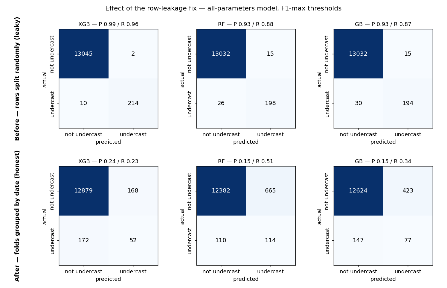
An initial analysis I performed showed ~0.8 precision. That number came from row leakage: folds were split by row rather than by date, so when a given forecast-hour row was scored, the other ~23 rows from the same day were sitting in the training set. The model didn’t have to forecast an undercast — it only had to recognize a day's conditions it had already memorized.
Below is that first-pass model evaluated both ways, each panel at its own F1-maximizing threshold. The top row is the leaky split, the bottom row is the date-grouped one. Reproducing the old split looks even better than the original writeup claimed — 0.9+ precision with nearly all undercast days caught — while the same model, same data, same algorithms scored honestly lands near 0.2 precision and misses most events. The old numbers were never forecast skill, just memorized days.
Note, this is the only data on this page still drawn from the first pass, so these numbers are not consistent with any other analysis in this writeup. The current pipeline groups folds by week and separates the holdouts by date, so the leaky split it illustrates cannot occur.
Model Results
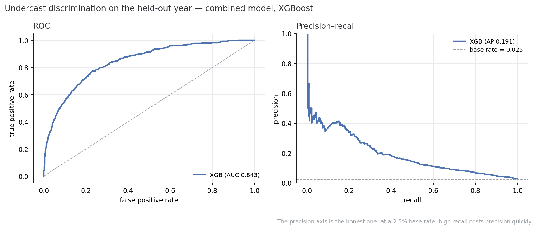
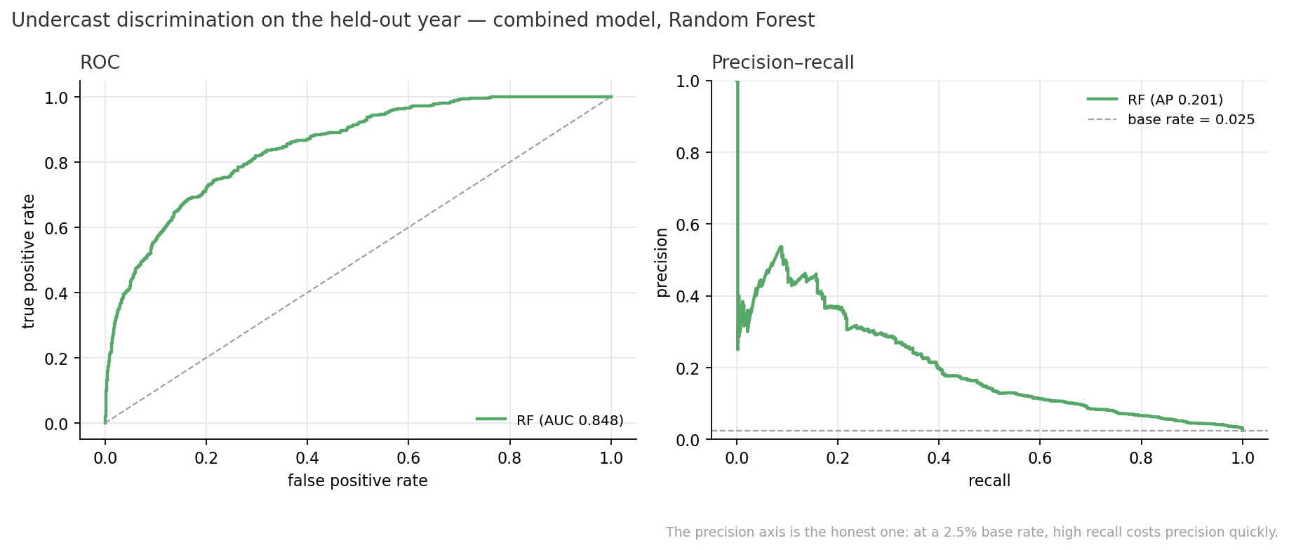
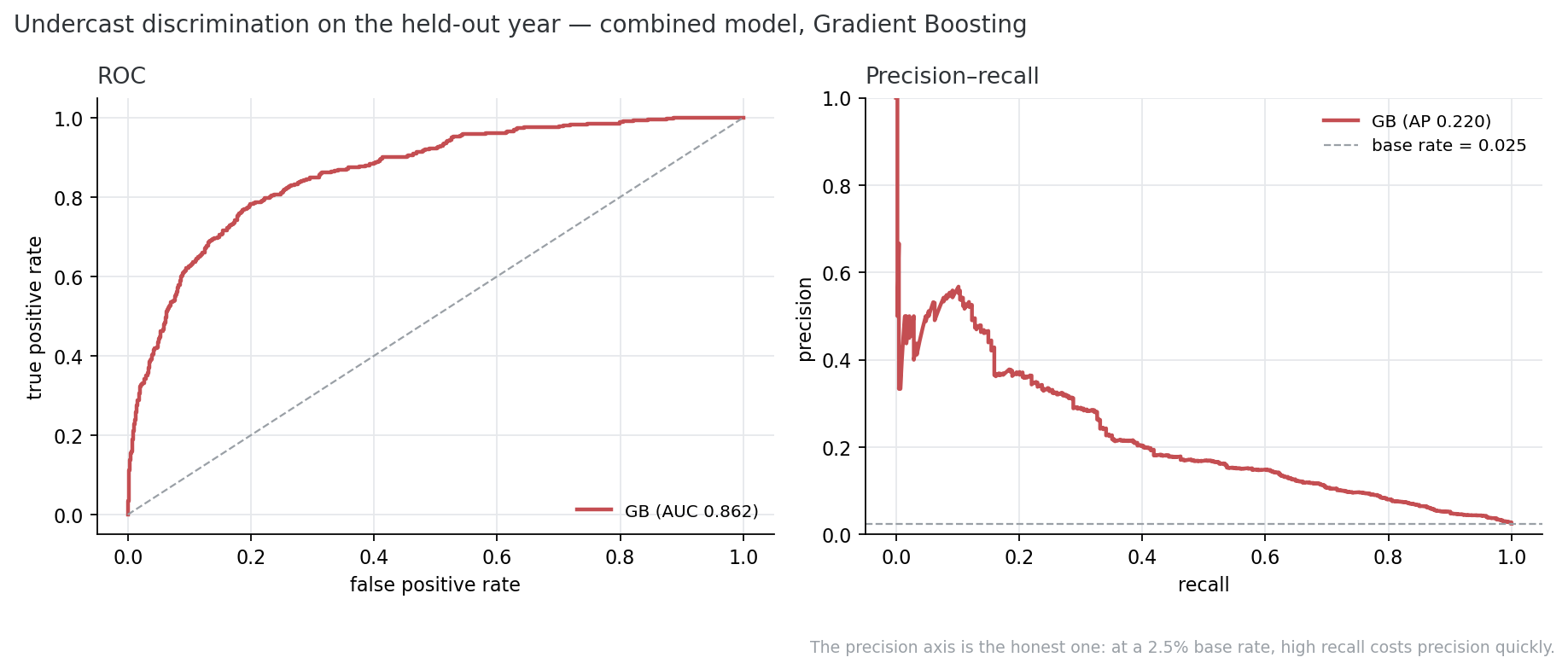
ROC and precision–recall curves for the combined all-parameters model on the held-out year, one panel per algorithm. The three algorithms finish within 0.03 ROC-AUC of each other.
Top features
The top features for each model are shown below.
Note that this doesn't mean a ton nor is it particurarily interpretable, as as many parameters are, if not degenerate, strongly correlated. We investigate this in a later section.
Accuracy over Forecast Lead
A 1 hour forecast isn’t particularly useful; a 10 day forecast can’t be trusted. In the section below, I evaluate the performance of the model as a function of forecast lead. Each row in the testing holdout is a forecast made 1, 24, 48, 72, 96, 120 or 144 hours before the hour it describes, and the same model is used at all seven forecast lead points. Each lead gets its own F1-optimal threshold, fitted on the true-base-rate holdout.
All figures below are for Gradient Boosting. ROC-AUC is on the full unsampled holdout year.
| Source | 1 h | 24 h | 48 h | 72 h | 96 h | 120 h | 144 h |
|---|---|---|---|---|---|---|---|
| Combined | 0.941 | 0.922 | 0.880 | 0.857 | 0.824 | 0.775 | 0.764 |
| RAP | 0.890 | 0.859 | 0.804 | — | — | — | — |
| HRRR | 0.889 | 0.870 | 0.837 | — | — | — | — |
| ECMWF | 0.879 | 0.872 | 0.842 | 0.847 | 0.804 | 0.739 | 0.754 |
| NAM | 0.861 | 0.830 | 0.818 | — | — | — | — |
| NBM | 0.844 | 0.769 | 0.762 | 0.734 | 0.690 | 0.675 | 0.651 |
| GFS | 0.842 | 0.818 | 0.790 | 0.747 | 0.745 | 0.682 | — |
| Lead | Threshold | ROC-AUC | Precision | Recall | Reads as |
|---|---|---|---|---|---|
| 1 h | 0.88 | 0.941 | 0.74 | 0.38 | 3 of every 4 undercast predictions are right |
| 24 h | 0.84 | 0.922 | 0.39 | 0.39 | about 2 in 5 |
| 48 h | 0.81 | 0.880 | 0.30 | 0.41 | about 1 in 3 |
| 72 h | 0.82 | 0.857 | 0.33 | 0.28 | about 1 in 3 |
| 96 h | 0.73 | 0.824 | 0.22 | 0.35 | about 1 in 5 |
| 120 h | 0.78 | 0.775 | 0.20 | 0.20 | about 1 in 5 |
| 144 h | 0.62 | 0.764 | 0.08 | 0.48 | about 1 in 12 |
Unsurprisingly, accuracy degrades with lead time. While ROC-AUC falls slowly, the precision drops quickly as lead time increases.
Two things are worth pulling out of the first table. Combining sources beats every individual one at every lead, and the margin widens with distance: at 1 h the best single source is within 0.05 AUC of the combination, by 120 h the gap is 0.09 even though only three models still reach that far.
Skill against forecast lead
As seen below, all metrics (save for precision) fall steadily over time.
Confusion matrices
Confusion matrices on the held-out year for each selected source, plus the 2-of-3 vote — a majority of the three hard calls, each made at its own threshold, not an average of their probabilities.
Pick a forecast lead to see how the same model degrades with distance. A single lead is scored at that lead’s F1-optimal threshold, while all leads” pools every row and uses the single global threshold.
Which ML model is best?
I chose to test three different ML models (and the consensus model), because it was cheap and it wasn't initially clear to me which model would have the best performance. As seen in the analysis above, the precision, recall, and ROC-AUC are pretty similar across all models.
Considering just the consensus model, an ensemble only pays when its members make different mistakes. If they agree, the vote can never overturn anything and all it does is average three copies of one opinion. So the first thing to look at is not the score but the agreement.
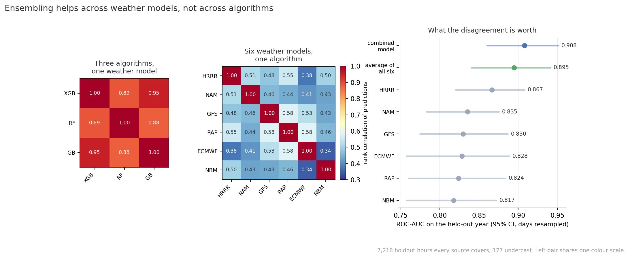
1. The model consensus vote does not help
On the combined model, at each member’s F1-optimal threshold:
| Held-out year | Webcam days | |||||
|---|---|---|---|---|---|---|
| Predictor | P | R | F1 | P | R | F1 |
| XGBoost alone | 0.26 | 0.29 | 0.27 | 0.35 | 0.18 | 0.24 |
| Random Forest alone | 0.28 | 0.31 | 0.30 | 0.25 | 0.06 | 0.10 |
| Gradient Boosting alone | 0.28 | 0.32 | 0.30 | 0.41 | 0.25 | 0.31 |
| Any of the three | 0.22 | 0.39 | 0.28 | 0.36 | 0.28 | 0.32 |
| 2 of 3 — the vote | 0.31 | 0.30 | 0.30 | 0.38 | 0.17 | 0.23 |
| Unanimous | 0.37 | 0.24 | 0.29 | 0.28 | 0.05 | 0.09 |
| Mean of the three probabilities | 0.28 | 0.31 | 0.29 | 0.31 | 0.14 | 0.19 |
Held-out year: 16,690 observations, 413 undercast. Webcam days: 4,122 observations, 154 undercast by human scoring.
It's pretty clear we're just playing with noise. All models have very similar performances, and there's no measurable benefit to any sort of ensemble.
2. Nothing else does better either
For kicks, I had ML try a couple other things as well. They all have similar performances. It seems pretty clear that fancier algorithms aren't providing any added benefit.
ML for idiots — and what the four alternatives are (click to expand)
Random Forest, deeper trees. The tuned forest with its depth cap raised. Same algorithm, more room per tree to keep splitting — the check on whether the forest was being held back by how short its trees were.
Histogram Gradient Boosting. Gradient boosting that first sorts each feature into about 256 buckets, so choosing a split becomes a histogram lookup instead of a scan over every distinct value. Much faster on wide data, and it treats “missing” as a direction it can split on rather than something to fill in first.
Extra Trees. Extremely randomised trees. Like a random forest, except the split thresholds are drawn at random instead of being optimised. Each tree is worse and the ensemble is less prone to memorising, which sometimes wins and here does not.
Logistic regression. Not a tree at all: a weighted sum of the inputs pushed through an S-curve to give a probability. It cannot represent an interaction between two parameters unless you build that interaction by hand, which is exactly what makes it the useful baseline — whatever it gets is available without any of the tree machinery.
| Algorithm | Combined, held-out year | HRRR, held-out year |
|---|---|---|
| Gradient Boosting (vote member) | 0.862 | 0.866 |
| Random Forest, deeper trees | 0.849 | 0.855 |
| Random Forest (vote member) | 0.848 | 0.862 |
| XGBoost (vote member) | 0.843 | 0.863 |
| Logistic regression | 0.819 | 0.861 |
| Histogram Gradient Boosting | 0.819 | 0.854 |
| Extra Trees | 0.799 | 0.850 |
ROC-AUC on the held-out year. Histogram Gradient Boosting gets the raw columns with their gaps intact, since it splits on missingness natively; logistic regression gets median imputation and standardisation, because handing a linear model the −9999 sentinel the trees use would let one fill value swamp every coefficient.
3. The disagreement that matters is between weather models
However, the diffeerent weather models do disagree in different ways. I chose to investigate six different models, precicely because they have distinct physics and different resolutions. It makes sense that a 3 km regional and a global model at 0.25° will give different results, and provide new information.
The combined model reaches 0.908 [0.860, 0.951]. Against the six-way average that is +0.013 [+0.003, +0.026]; an improvement, but only slightly.
All models are effectively the same
There's no benefit to a vote, ensemble, or comparing different models from here on out. A single combined-source model with per-lead thresholds is as good as any ensemble. From here on out, I use Gradient Boosting.
Are we overfitting?
The combined model reads 213 feature columns, and the training split holds 31,009 rows. However, not all features or rows are independent.
Rows are not observations
Each undercast hour enters the training set once per forecast lead, but multiple observations from the same undercast event and not indipentent. They're not the same data point either though. Assuming the points are fully degenerate, we find our actual training set is reduces as follows:
| Counting unit | n | Per feature |
|---|---|---|
| Positive rows | 5,572 | 26.2 |
| Distinct positive valid hours (de-duplicating the seven leads) | 797 | 3.7 |
| Distinct undercast episodes (gaps up to 2 h bridged) | 182 | 0.85 |
| Distinct undercast days | 175 | 0.82 |
Against 213 feature columns, the usual rule of thumb of ten events per parameter is off by more than an order of magnitude. We have more features than undercast days! However, feature columns are also strongly correlated and contain some degeneracies.
Some features are strongly correlated
213 columns is not 213 independent knobs. The combined model is six weather models’ columns stacked side by side, meaning a parameter such as the temperature at 500mb tmp_500mb, has six different versions: tmp_500mb_hrrr, tmp_500mb_gfs, tmp_500mb_nam, tmp_500mb_rap and tmp_500mb_ecmwf.
Clearly all six versions are going to be highly correlated, though some models perform better than others, which is why the combined model does better. Removing all duplicate parameters(across models), the 213 columns collapse to 78 distinct physical quantities, plus four calendar encodings (month and hour as sine/cosine). Forty-one of those quantities are carried by more than one source and the remaining thirty-seven are published by a single model.
When evaluating the correlation between same-quantity pairs, we find that the median is 0.872, against 0.181 for a randomly drawn pair of different quantities.
All 300 same-quantity, different-source pairs, binned by |Spearman r|. The dashed outline is the baseline: 19,317 randomly drawn pairs of different quantities, shown as a share of its own distribution so the two are comparable.
Performing principal component analysis on the on the 11,620 training rows where every source reports, over the 98 columns populated more than half the time, 29 components carry 95% of the variance and 21 carry 90%; the participation ratio is 8.7. There's more analysis that could be done here on parameter degeneracy, and which components are most important, but for now it seems the risk of over-training our model is low.
As seen in the two plots below, there's no clear benefit to trimming the model parameters or limitting the tree depth.
Each budget is the top k features by importance, retrained and scored on both untouched holdouts, plotted as change against the full 213-feature model. The grey band is the noise floor — ±0.005, the spread of the current configuration under five seeds.
Same construction as the chart above: change against the current configuration, with the ±0.005 reseed band.
Final Model
Combining everything, the highest-performing model is:
- Uses data from all weather models, not just one.
- Uses Gradient Boosting, since an ensemble does not improve performance.
- Keeps all features and trims it to a depth of 3; see overfitting and capacity checks.
Confusion matrices are shown below for each lead.
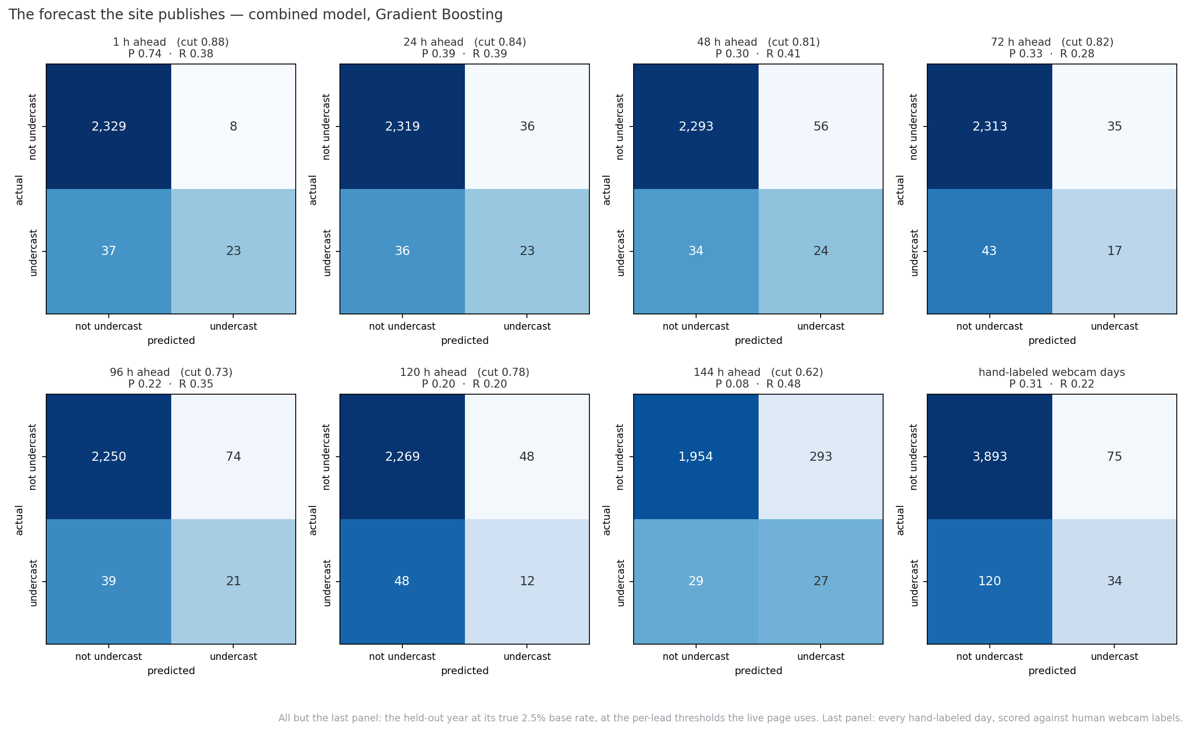
| How far ahead | When it says undercast, it’s right | Of real undercasts, it catches | ROC-AUC |
|---|---|---|---|
| 1 hour | 74% | 38% | 0.941 |
| 24 hours | 39% | 39% | 0.922 |
| 48 hours (2 days) | 30% | 41% | 0.880 |
| 72 hours (3 days) | 33% | 28% | 0.857 |
| 96 hours (4 days) | 22% | 35% | 0.824 |
| 120 hours (5 days) | 20% | 20% | 0.775 |
| 144 hours (6 days) | 8% | 48% | 0.764 |
Held-out year, true 2.5% base rate, each lead at its own threshold.
Next Steps
You're only as good as your data, and our data is adequate at best. The model would benefit from a larger, and more accurate dataset. Any sort of additional data that could help with identifying historical undercast conditions would go a long way.
Might also be interesting to look into parameter importance more, and understand why different models perform better/worse, and what primary factors drive undercast conditions.
AI usage
The vast majority of the coding was done with AI. I made all high-level model design decisions and reviewed all analysis steps made by AI. AI was particularly helpful when it came to ML implementations and web visualizations, while it struggled with physics/weather interpretations and higher-level analysis and reasoning. The vast majority of the text on this page was written by me, with small sections of AI generated text (eg. for an overview of ML models).
Data availability
All scripts used for this analysis are available on GitHub. For access to the data, or with any questions, contact me at ehingerl@mit.edu.